Using the workbench
The workbench is where you assemble and run an experiment. This guide shows where to find its controls and how adding a block, connecting it and starting it fit together. If MOSAIC is not running yet, begin with Getting Started.
Find your way around
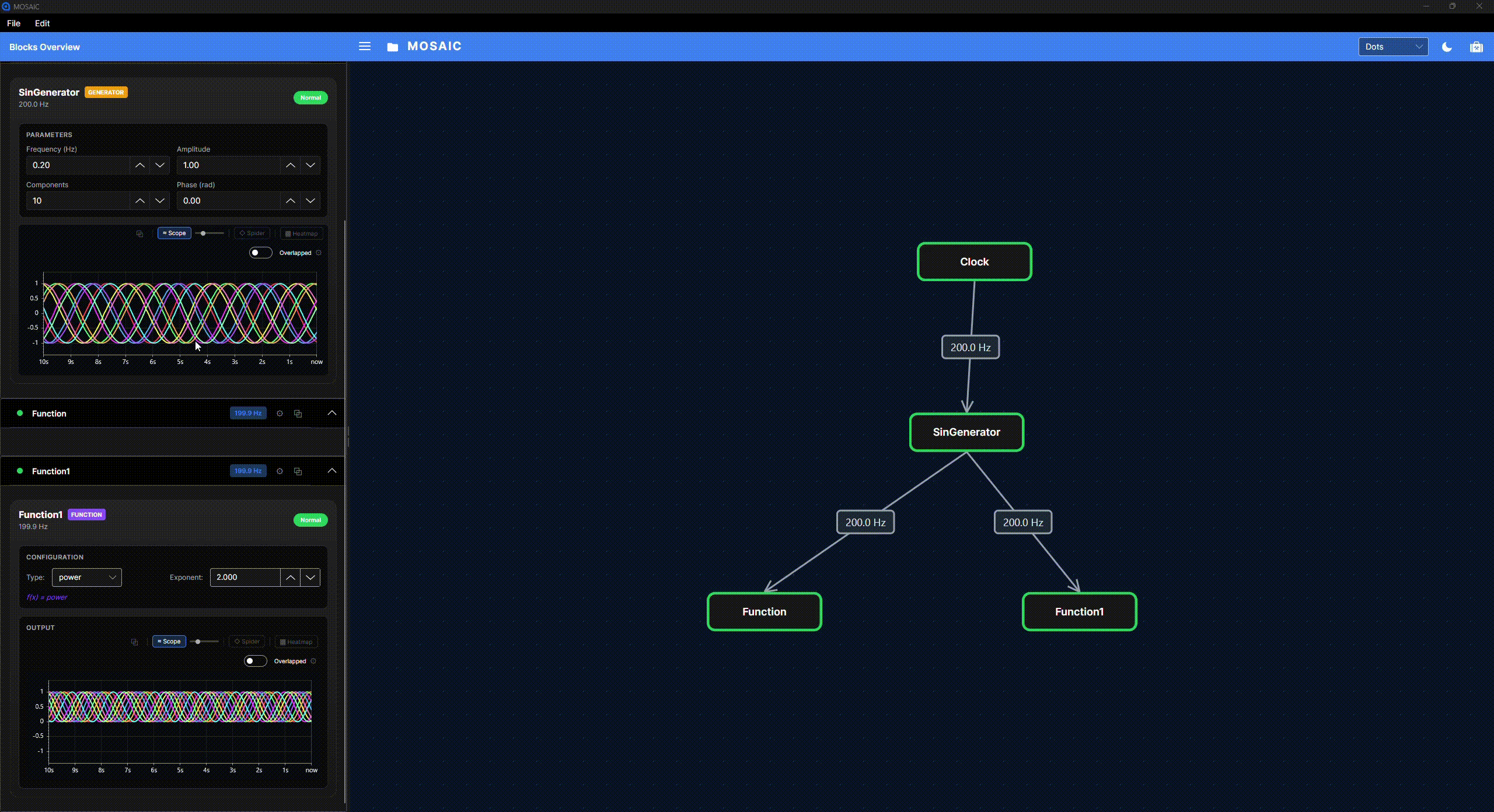
The recordings on this page come from a desktop teaching session. They demonstrate the controls; block names and settings can differ from the downloadable tutorials. Select Play animation to watch a demonstration, and Stop animation to return to its still image. Use View full-size animation to open the original recording in a new tab, where you can enlarge it to read the controls. The written steps also explain each action.
| Area | What you do there |
|---|---|
| Top toolbar and File menu | Open a pipeline or save your arrangement and settings. |
| Centre: canvas | Place blocks and connect their ports to define where data goes. |
| Right: block palette | Find an available block and add an instance to the experiment. |
| Left: Blocks Overview | Expand a block's card to change settings, operate it or show its available plots. |
The canvas and cards refer to the same blocks. Moving a node makes the graph easier to read; changing a parameter changes what that block does. A plot shows the data selected for that block's visualization.
Open an existing experiment
Choose File → Open, or the folder button, and select a pipeline JSON file. For a hardware-free starting point, use the example in Your First Pipeline. Check that the expected blocks and connections loaded before starting the source. Resolve loading errors first: a partially loaded graph may not represent the intended experiment.
Opening a pipeline restores its setup. For a clock-driven example, you still need to press Play in the Clock card. Device-based experiments also need a live device connection; reopening a file does not establish that connection for you.
Add a block
- Pause the source while changing the graph.
- Find the operation in the right-hand palette. Use the Block Catalogue when you need to check its purpose, parameters or required inputs.
- Drag the operation onto the canvas. Give the new block a distinct name and confirm the settings in the creation dialog.
- Find the resulting node on the canvas and its controls in Blocks Overview.
Adding an instance gives it a place in the experiment; connecting that instance to its input data is a separate step. The palette reflects the current platform and build options, so optional device blocks may not appear.
Connect it to the data it needs
In the graph's build mode, drag from an upstream block's bottom output port to the next block's top input port. The dashed line follows the pointer during the drag. A completed connection means that values published upstream are passed to the receiving block. One output can feed several downstream blocks.
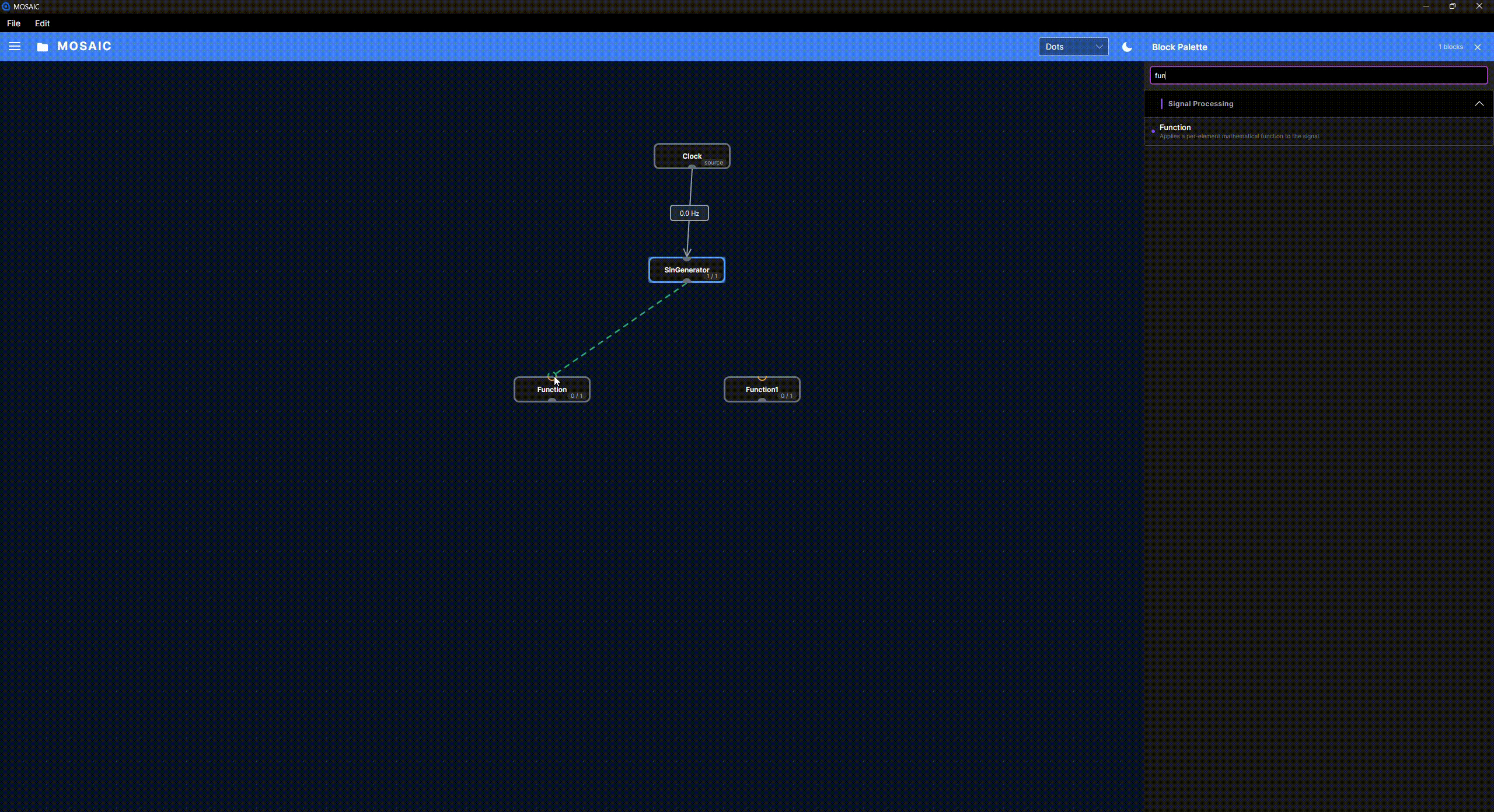 View full-size animation (new tab)
Check the receiving block's input requirements. Acceptance by the editor does not guarantee that the values have the right shape or meaning. For example, a feature calculation may need a window of samples, while another operation needs one vector. The block reference explains these requirements; Data Shapes and Time explains how the forms differ.
Change settings and start the source
Expand the appropriate card in Blocks Overview. Controls depend on the block: a Clock has a rate and Play/Pause controls; a signal generator has waveform settings; a Function exposes settings for its selected operation, such as a multiplication factor. Apply the change if the control provides an Apply action, then resume the source.
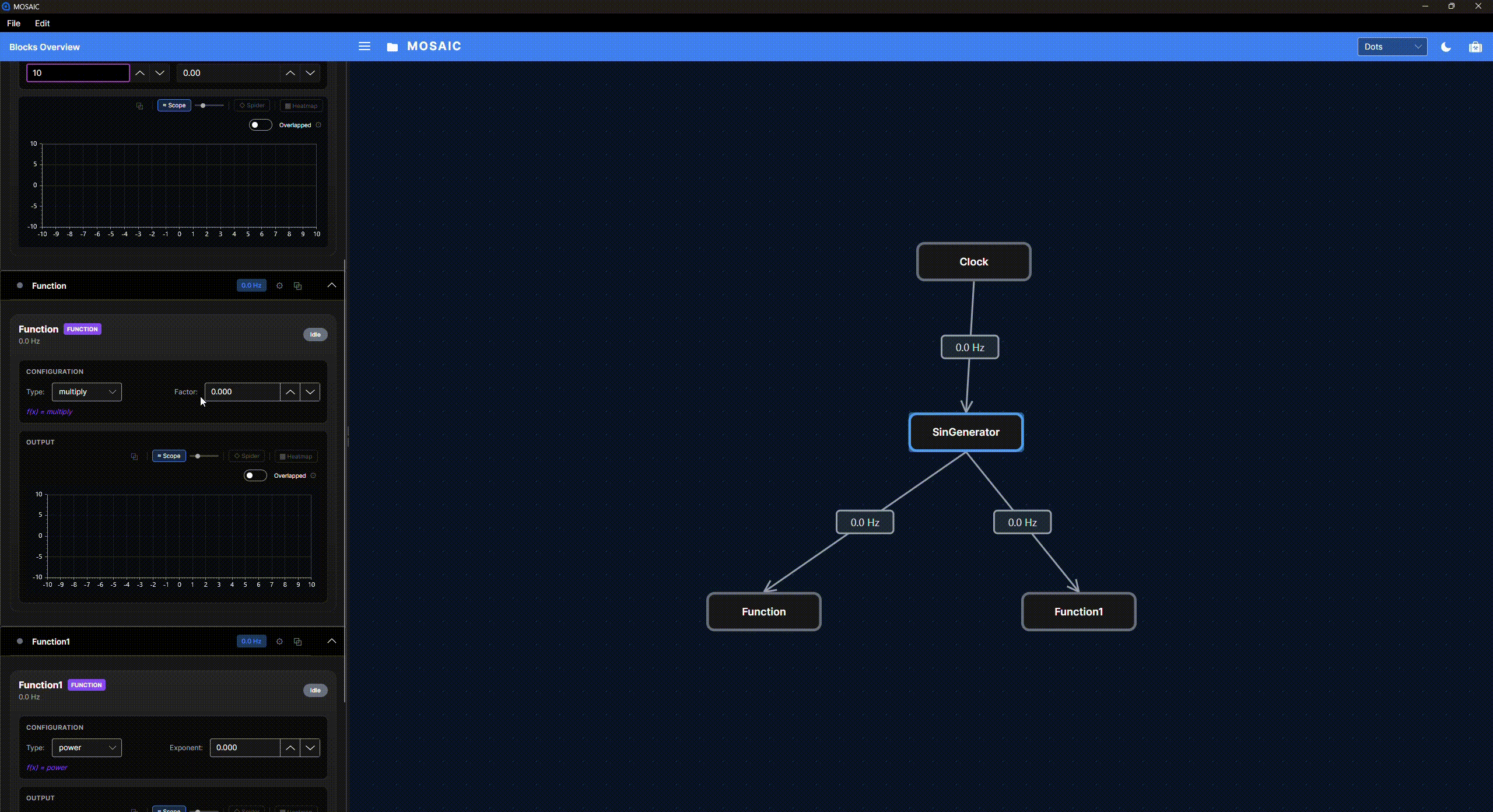 View full-size animation (new tab)
For this clock-driven graph, pausing the Clock stops new generated samples. Other source blocks can have their own connection or start controls. The Clock is not a universal start/stop switch for independent network streams or workers.
Inspect the source first, then follow the connections downstream. A displayed rate or a green connection alone does not prove that a sensor is supplying fresh, meaningful measurements. Check the connection status and the values themselves.
Compare results, then save
Show a card's Scope or another available monitor to inspect its data. On desktop, the pop-out control lets you move a view into a separate window for comparison. See Reading the Plots for a demonstration. Some blocks have no dedicated plotting card.
Use File → Save As to keep your experiment setup. Recording numerical data is a separate action: choose what to record and where to save it as described in Recording and Saved Pipelines. Saving the graph does not save the whole live session, plot history or every block's learned state.
Continue with Your First Pipeline for an exercise with specific settings and expected results.